In some version (64 bits) you need to change the path of the help file in order to launch it on the desktop. It must be :
"C:\Program Files (x86)\Rhythms". Change is in : Environment options / Directories / Help file (Uncheck allows changing the help file directory) and so on.
You can also select a directory to store your data files (Above "help file" : "Data")

Entry of data into the software can be done in two ways : From an Excel (Microsoft registered) file converted into .txt file. Directly in the integrated editor. Both is explained in the help file. With the editor, it is easy to gather data and if there is an error in catching the data the error is explained.

You can choose the size of your chart in the Environment Menu Options/Graphics/Publishing Window. You can also choose the type of data points, the text size. The size of the lines. Here it's important to spend time to try different options.

In every chart it is very important to try the "right click" as there are different options : To save the graphic for example but also properties where you can control the graphic : color, size, scales etc.

Some scientific journals publishers ask for denser graphics. You must save the graphic (often right click on the graph !) in a directory and call it in Paint Shop Pro (registered), Photo Shop (registered), or even in a small image free editor like Paint.net (registered) or the free Gimp (registered) where you can increase the density of the picture.

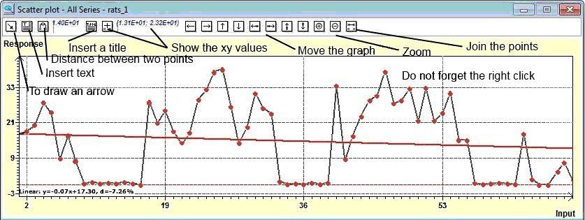
There are various tools on the chart. You can change the size, trace an arrow, insert text, write a title, calculate the distance between two points, insert values, move the graph, zoom in, zoom out, join the points (see the figure below).

Petit rectificatif historique: Le périodogramme de Lomb and Scargle est en fait le périodogramme de Scargle (The Astrophysical Journal, 263:835-853, 1982 December 15) C'est nous, semble-t-il, il y a déjà quelques temps qui l'avions appelé comme cela...
Quant à l'origine du Cosinor c'est un grand mystère malgré notre "grande" connaissance du sujet. Cela remonte aux années 60... (On trouve : Halberg F, Engel R, Swank R, Seaman G, Hissen W. Cosinor-Auswertung circadianer Rhythmen mit niedriger Amplitude im menschlichen Blut. Physik Med u Rehab 1966;5:101-107., Halberg F., Tong Y.L. & Johnson E.A. (1967). Circadian system phase - an aspect of temporal morphology; procedures and illustrative examples. In The Cellular Aspects of Biorhythms, pp.20-48, ed. VONMAYERSBACH, H. NewYork : Springer) Il y a différentes écoles (de calculs et de résultats) Ici nous utilisons la méthode Américaine de Halberg et Coll.

1 - Detrend data to have a stationary set of data. We'll choose linear detrend. For exemple the trend is : -0.07x + 17.3 (see the previous figure)

2 - Search the period close to 24 hours or more in this example.

The difference in the determination of the period value becomes that for the RES we take the mean vector and the others periodogram we take all data. The RES is the more close to the period (Population Mean Cosinor means different subjects)

3 - Modelize data by a cosine function (Population Mean Cosinor)

Remains that the model equation is now : -0.07x + 17.3 + 1.47E+01Cos((2Pit/25.90)-5.77E+00)+1.62E+01

Because it is intended to be represented on the confidence ellipse which is graduated in negative degrees in the direction of clockwise.

If you want to have a positive acrophase :

- In radians add 2Pi
- In degrees add 360

If you want an acrophase in hours minutes just make the rule following :

360 degrees -> 24 hours (the period)
x degrees -> y in hours

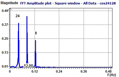
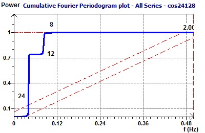
Because we need to study one periodicity (24 hours for the Chronobiology data) We have to remove the others periodicities. In this case we can use the Hodrick-Prescott filter. For example we take a set of Chronobiologic data of three periods 24, 12 and 8 hours. We often find this case of set of data in Chronobiologic biological time series.

The aspect of this set of data is given by the Scatter plot and the spectral analysis by the Scargle periodogram and the Jenkins and Watts periodogram :

After filtering with the Hodrick-Prescott filter. We can see two periodicities :

After filtering again with the Hodrick-Prescott filter. It remains only the 24 hours periodicity :

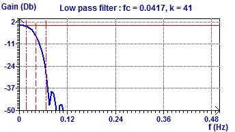
The aim is also to separate the periodicities... With a cut off frequency of 24 hours (0.0417 Hz) we can keep one frequency of 24 hours (see the previous scatter plot). The Filter and the Fourier Transform.

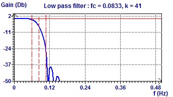
With a cut off frequency of 12 hours (0.0833 Hz) we can keep two frequencies of 24 and 12 hours (see the previous scatter plot). The Filter and the Fourier Transform.

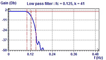
With a cut off frequency of 8 hours (0.125 Hz) we can keep three frequencies of 24, 12 and 8 hours (see the previous scatter plot). The Filter and the Fourier Transform.

Example of Plasma Melatonin (3 main periods found : 24, 12, 8)